Epidemiology is “the study of disease in populations and of factors that determine its occurrence over time.” The purpose is to describe and identify opportunities for intervention. Epidemiology is concerned with the distribution and determinants of health and disease, morbidity, injury, disability, and death in populations. For veterinary epidemiology, this intervention is to enhance not only health but also productivity. Distribution implies that diseases and other health outcomes do not occur randomly in populations; determinants are any factors that cause a change in a health condition or other defined characteristic; morbidity is illness due to a specific disease or health condition; mortality is death due to a specific disease or health condition; and the population at risk can be humans, animals, or plants.
Epidemiology is applied in many areas of human and animal health practice. Among the most salient are to observe historical health trends to make useful projections into the future; discover (diagnose) current health and disease burden in a population; identify specific causes and risk factors of disease; differentiate between natural and intentional events (eg, bioterrorism); describe the natural history of a particular disease; compare various treatment and prevention products and techniques; assess the impact, efficiency, cost, and outcome of interventions; prioritize intervention strategies; and provide foundation for public policy.
Epidemiological Terms and Concepts
The natural history of a disease in a population, sometimes termed the disease’s ecology, refers to the course of the disease from its beginning to its final clinical endpoints. The natural history begins before infection (prepathogenesis period) when the agent simply exists in the environment, includes the factors that affect its incidence and distribution, and concludes with either its disappearance or persistence (endemnicity) in that environment. Although knowledge of the complete natural history is not absolutely necessary for treatment and control of disease in a population, it does facilitate the most effective interventions.
An important epidemiological concept is that neither health nor disease occurs randomly throughout populations. Innumerable factors influence the temporal waxing and waning of disease. A disease is considered endemic when it is constantly present within a given geographic area. For instance, rabies in animals is endemic in the US. An epidemic occurs when a disease occurs in larger numbers than expected in a given population and geographic area. Cases of rabies caused by the raccoon-associated variant of rabies virus were considered an epidemic throughout the eastern US for much of the 1980s and 1990s. A subset of an epidemic is an outbreak, when a greater occurrence of cases of disease than would normally be expected occurs in a smaller scale (eg, an outbreak of feline panleukopenia virus in an animal shelter). Finally, a pandemic occurs when an epidemic becomes global in scope (eg, 1918 influenza pandemic or COVID-19 pandemic).
The population at risk is those members of the overall population capable of developing the disease or condition of interest. This concept of population at risk seems simple, but misinterpretations can lead to erroneous study results and conclusions. For example, a study of ovarian cancer among animals in a population should not include male dogs in the population at risk (frequently expressed as the denominator in an epidemiological ratio).
A ratio is the value obtained from dividing one quantity by another (X/Y). The numerator and denominator may be independent of each other. In fact, in epidemiology, the term ratio is applied when the numerator is not a subset of the denominator. For example, in a class of veterinary students in which 88 are female and 14 are male, the gender ratio of female students to male students is 88/14, or 6.3 to 1.
A proportion is a type of ratio in which the numerator is part of the denominator (A/[A + B]). Therefore, they are not independent. For example, suppose that, among domesticated dogs testing positive for internal parasites in Knoxville, Tennessee, 889 were male and 643 were female. The proportion of female dogs among those found to have parasite infections would be 643/(889 + 643), or 0.42.
A rate is another type of ratio in which the denominator involves the passage of time. Rates can be used to measure the speed of a disease event or to make epidemiological comparisons between populations over time. Rates are typically expressed as a measure of the frequency with which an event occurs in a defined population in a defined time (eg, number of foodborne Salmonella infections per 100,000 people in the US per year).
Incidence is a measure of the new occurrence of a disease event (eg, illness or death) in a specified population within a defined time period. Two essential components are the number of new cases and the period of time in which those new cases appear. Although incidence can be expressed as a simple count of the number of new cases of disease observed in a population, it is more useful as a measure of disease frequency when expressed as a rate. For example, in a class of 102 veterinary students, if 13 of them developed influenza over the course of an academic quarter, the incidence rate would be 0.127 cases per student per quarter (or 12.7 cases per 100 students per quarter). An attack rate is an incidence rate; however, the period of susceptibility is very short (usually confined to a single outbreak).
Measures of Disease Occurrence
Term | Definition/Explanation | Formula | Sample Calculation |
|---|---|---|---|
Prevalence | Prevalence is the proportion of existing cases of disease present in a designated population at a given point in time. Usually, prevalence refers to a “point prevalence” (ie, the prevalence at one point in time). | Prevalence is calculated as the number of cases at a designated time divided by the number of individuals at risk at the designated time; it is usually expressed as a percentage. Prevalence = (No. of cases / PAR) x 100% | At a single point in time (eg, based on the results of a serosurvey of dogs in the practice area), 237 dogs of 6,821 dogs with active records in a practice had coccidioidomycosis. In this scenario, the prevalence of coccidioidomycosis at the time of the serosurvey would be 3.5%. Prevalence = (No. of cases / PAR) × 100% = (237 / 6,281) × 100% = 0.035 × 100% = 3.5% In a class of 102 veterinary students, 7 were married at the start of year 1. In this scenario, the prevalence of married veterinary students in a class at the start of year 1 would be 6.9%. Prevalence = (No. of cases / PAR) × 100% = (7 / 102) × 100% = 0.069 × 100% = 6.9% |
Period prevalence | Period prevalence differs from point prevalence in that it includes the number of existing cases at the start plus new cases that occurred in a designated population during a time interval of interest. | Period prevalence = (No. of cases [preexisting + new] / PAR) × 100% | In addition to 237 dogs with known coccidioidomycosis, the practice diagnosed 542 clinical cases in a particular year among their patient population of 6,821 dogs. In this scenario, the period prevalence of coccidioidomycosis for the year would be 11.4%. Period prevalence = (No. of cases [preexisting + new] / PAR) × 100% = (237 + 542) / 6,821 × 100% = 0.114 × 100% = 11.4% |
Incidence | Incidence is the number of new cases of a disease in a population that is at risk (and disease-free) within a specified period of time. | Incidence is calculated as the number of newly diagnosed cases divided by the total population at risk over a specified period of time. Incidence can be calculated as incidence risk (cumulative incidence) or a true rate (incidence density). | |
Cumulative incidence (incidence risk) | Cumulative incidence (also called incidence risk or incidence proportion) quantifies the risk of new disease occurrence (ie, the probability of an animal developing a disease in a defined time period). Case-fatality rate is a cumulative incidence for death due to a given cause. | Cumulative incidence is calculated as the proportion of animals developing a disease in a defined time period; it is usually expressed as a percentage. Cumulative incidence = (No. of new cases in time period / PAR) × 100% | On a small dairy farm with 102 cows, 13 developed ketosis over the course of a year. In this scenario, the cumulative incidence would be 12.7% per year. In other words, the estimated probability (incidence risk) that a lactating dairy cow develops ketosis over the next year is 12.7%. Cumulative incidence = (No. of new cases in time period / PAR) × 100% = (13 / 102) × 100% = 0.127 × 100% = 12.7% per year Note that it is essential to quote the relevant time period as part of the cumulative incidence (ie, the risk of developing disease over the next year or the next week are very different). |
Attack rate | In outbreak investigations, attack rate is often used as a measure of disease frequency. Note that attack rate is not a true rate but actually a proportion. | Attack rate is calculated as the cumulative incidence of disease in outbreak situations. Attack rate = (No. of new cases since onset of outbreak / PAR at onset of outbreak) × 100% | In an outbreak of upper respiratory disease, 53 out of 77 cats in a municipal shelter became infected. In this scenario, the attack rate is 69% during the outbreak. Attack rate = (No. of new cases since onset of outbreak / PAR at onset of outbreak) × 100% = (53 / 77) × 100% = 0.69 × 100% = 69% during outbreak |
Incidence density (incidence rate) | Incidence rate quantifies the rate at which new events occur in a population. | Incidence rate is calculated as the number of new cases in a population divided by animal-time at risk during a given time period. There are several methods of calculating animal-time at risk (eg, the sum of each animal’s time at risk or average population during the time interval). Incidence rate = No. of new cases / Total animal-time of observation | Of 50 laboratory gerbils (Meriones unguiculatus) kept in a biomedical research facility, 25 developed aural cholesteatomas by 2 years of age. In this scenario, the incidence rate is 2.5 cases / 10 gerbil-years. Incidence rate = (No. of new cases / Total animal-time of observation) = 25 cases / (50 gerbils x 2 years each) = 0.25 cases / gerbil-year = 2.5 cases / 10 gerbil-years Note that incidence rate is typically adjusted to have at least one digit to the left of the decimal place by applying a multiplier to both the numeric quantity and the units of animal-time. |
Incidence count | Simple count of the number of new cases of disease in a population. Without information about the population at risk, an incidence count can be misleading as a measure of disease frequency. | ||
PAR = Population at risk. The population at risk is defined by susceptibility to the condition of interest, time period of interest, geography, species, breed, age, sex, etc. | |||
A similar concept to incidence is prevalence. Usually, this refers to point prevalence: the total number of cases that exist at a particular point in time in a particular population at risk. If, at a given time during the academic quarter, 7 of 102 students had influenza, the prevalence would be 7/102 or 0.069 cases per class (or 6.9%).
Measures of disease burden typically describe illness and death outcomes as morbidity and mortality, respectively. Morbidity is the measure of illness in a population, and numbers and rates are calculated in a similar fashion as with incidence and prevalence. Mortality is the corresponding measure of death in a population and can be applied to death from general (nonspecific) causes or from a specific disease. Mortality from a particular disease is expressed as the case fatality rate (CFR), which is the number of deaths due to that disease occurring among affected individuals in a given time period.
In another example, consider a large veterinary practice in the southwestern US that frequently sees dogs with coccidioidomycosis. The practice diagnosed 542 clinical cases in a particular year, 83 of which died from the disease in the course of that year. The month in which the most cases were diagnosed was September, in which 97 cases were diagnosed. Further, at a single point in time (perhaps based on the results of a serosurvey of dogs in the practice area), 237 dogs of 6,821 dogs with active records in the practice had the disease. In this scenario, the prevalence of coccidioidomycosis at the time of the serosurvey would be 237/6,821, or 0.035 (3.5%); the incidence count in September would be 97 cases, and the incidence rate would be 97/6,821, or 0.014 (1.4%). Finally, the annual mortality rate observed in that practice due to coccidioidomycosis would be 83/6,821, or 0.013 (1.3%), and the case fatality rate would be 83/542, or 0.153 (or 15.3%).
Medical surveillance is the analysis of health information to look for problems that require targeted prevention. Foreign animal disease surveillance is conducted by the Veterinary Services division of USDA's Animal and Plant Health Inspection Service (APHIS), with its vast network of state and private-practice veterinarians, to detect threats to animal health in a timely manner. Public health surveillance is the ongoing systematic collection, analysis, interpretation, and dissemination of outcome-specific data essential to the planning, implementation, and evaluation of public health practice. In epidemiology, health surveillance is accomplished in either passive or active systems.
Passive surveillance occurs when individual health care providers or diagnostic laboratories send periodic (in accordance with state or federal regulations) reports to the public health agency. Because this reporting is voluntary (sometimes referred to as being "pushed" to health agencies), passive surveillance tends to underreport disease, especially in diseases with low morbidity and mortality. Passive surveillance is useful for longterm trend analysis (if reporting criteria remain consistent) and is much less expensive than active surveillance. An example of passive surveillance is the system of officially notifiable diseases routinely reported to CDC by state, territorial, and other reporting jurisdictions across the US. Active surveillance, in contrast, occurs when epidemiologists or public health agencies seek specific data from individual health care providers or laboratories. In this case, the data are “pulled” by the requester, usually during emerging diseases or noteworthy changes in disease incidence. Active surveillance is usually much more expensive and labor intensive; it typically is limited to short-term analyses of high-impact events. An example is the multiyear, global surveillance effort to detect new cases of COVID-19 during the pandemic that began in 2020.
Descriptive Epidemiology
Given that neither health nor disease is equally distributed throughout a population, epidemiologists use various methods to study and describe their occurrence. In descriptive epidemiology, diseases are classified according to the variables of individual (person or animal), place, and time.
Individual (person or animal): Who is affected by this disease? Certain variables may highlight changes in disease status and can be used to focus additional studies and interventions. Common person variables include age, sex, race, socioeconomic status, marital status, religion, smoking status, etc. In the case of animals, equivalent variables may include signalment (age, species, breed, sex and reproductive status [eg, sexually intact vs neutered, pregnant vs nonpregnant]), function (eg, meat, milk, or fiber production; racehorse, working horse, or pleasure horse; companion dog vs military working dog), and wild or feral vs domesticated.
Place: Where does this disease occur? Place variables commonly illustrate geographic differences in the occurrence of a particular disease. Focused studies can help assist epidemiologists to determine why those differences have occurred and to identify specific risk factors. Common place variables include comparisons across national, state, and municipal boundaries and between urban and rural communities, and even specific venues for investigating disease outbreaks. For animal populations, “place” may refer to housing (eg, indoors vs outdoors, pen number or stall) or type of herd management (eg, intensive feedlot confinement vs extensive grazing). Place may also relate to risk of exposure to infectious animals at sale barns or during shipment or to external factors such as severe weather and natural disasters.
Time: When and over what time period (hours, days, weeks, day vs night) does this disease occur? Time variables are important to describe when disease occurs in relation to various factors of potential exposure and vulnerability. In animals, time may refer to milking shift, breeding season, lambing/calving season, at weaning, during shipment, on arrival at the feedlot, dry vs wet season, etc. Common time variables include secular trends (changes over long periods of time), seasonal/cyclic periods, and specific points in time (eg, outbreaks, epidemics, clusters, etc).
When a particular disease is observed relative to the variables of person, place, and time, it is often systematically described to facilitate more in-depth study. These systematic descriptions commonly take the form of case reports, case series, or cross-sectional studies:
Case reports are accounts of single or a few noteworthy health-related incidents (eg, an epidemiological description of a case of human rabies).
Case series are listings of larger numbers of cases, usually presented consecutively (eg, a characterization of dog bite incidents in a population of veterinarians or technicians over time). Case series articles are useful for comparing variables of person, place, or time as they appear to affect the occurrence of a particular disease.
Cross-sectional studies are one-time assessments of the incidence or prevalence of a disease in a defined population, which is usually selected at random from a larger population at risk (eg, a serosurvey of veterinarians for the presence of antibodies to Bartonella henselae organisms to determine risk factors and for cat-scratch disease). Cross-sectional studies are especially useful in forming hypotheses to be addressed by follow-on analytical studies.
Bias is any trend in the collection, analysis, interpretation, publication, or review of data that can lead to conclusions that differ from the truth. Two main types of bias in descriptive epidemiology are selection bias and observation bias:
Selection bias results from the identification of subjects or cases from a subset that is not representative of the entire population at risk. For example, data sourced from a veterinary teaching hospital may not be typical of the general population if a predominance of patients were referred for specialized care, have especially willing and capable owners, and have survived long enough to have a confirmed diagnosis.
Observation bias arises from systematic differences in the method of obtaining information from subjects or cases. For example, in a controlled trial, knowledge by investigators and owners of which animals are in the control group and which are receiving an active intervention can alter estimates of intervention effects.
In general, bias in descriptive studies is not as prevalent or consequential as bias in analytical studies.
In summary, descriptive epidemiology serves to describe the occurrence of disease in a population. Descriptive methods are commonly (but not always) applied to little-known diseases; they use preexisting data; address the questions of who, where, and when; and identify potential associations for more in-depth analytical studies.
Analytical Epidemiology
Analytical studies are applied to study the etiology of disease, to identify a causal relationship between exposures and health outcomes. They are typically used when insights of a particular health issue are available, commonly from previous descriptive studies. In evaluating the causality of disease associations, analytical studies address the question of “why” as opposed to the “person/place/time” of descriptive studies.
Once potential associations have been observed between those who have a particular disease and those who do not, further investigations are undertaken to determine causality and identify effective interventions. The first step in an analytical study is to form some conjecture regarding observed exposures and health outcomes. The null hypothesis states the default assumption that there is no association between the exposure in question and the disease outcome. This assumption of no association is made even though the epidemiologist often thinks that some association actually exists. Studies are designed to test the null hypothesis and either reject it (by finding significant evidence that some association actually does exist between exposure and disease outcome) or fail to reject it (by finding no significant evidence that an association exists).
Analytical epidemiology is accomplished through either observational studies or interventional studies. In observational studies, the investigator does not control the exposure between the groups under study and typically cannot randomly assign subjects to study groups.
Observational Studies in Epidemiology
Ecological Studies
The subjects of ecological studies are groups of humans or animals instead of individuals. The group has no size limitation but must be able to be defined. For instance, the group could be a kennel of dogs, a class of veterinary students, or the citizens of an entire country.
Once defined, the group is analyzed against some exposure to see what outcomes ensue. Examples of ecological studies include Dr. John Snow’s analysis of the association between the incidence of cholera in London and where people obtained their drinking water, an analysis of how tobacco taxes affect tobacco usage, and an analysis of certain occupations for resultant hearing loss.
Ecological studies have several advantages over other types of observational studies. They are relatively quick, easy, and inexpensive. Individual data are not necessary, only aggregate data for the groups under study. Finally, they are useful in generating information about the overall context of health, especially how it is affected by variables such as demographics, geography, and the social environment.
Ecological studies also have several disadvantages. First, the measurement of many exposures is imprecise, especially of large groups in which the influences of those exposures is difficult to define or not equally exerted. This phenomenon of unequal variable exertion results in another potential drawback to ecological studies known as ecological fallacy where associations observed at the group level do not necessarily hold true at the individual level. For example, aggregate data showing higher risk of heart murmurs in brachycephalic dogs than in non-brachycephalic dogs may not apply at the individual breed level due to large differences in individual breed predispositions to disorders. It would incorrect to infer that any given brachycephalic breed had a higher risk than any given non-brachycephalic breed.
In an epidemiological example of ecological fallacy, researchers found that death rates from breast cancer were notably higher in countries where fat consumption was high when compared with countries where fat consumption was low. This is an association for aggregate data in which the unit of observation is country. Thus, in countries with more fat in the diet and higher rates of breast cancer, women who eat fatty foods are not necessarily more likely to get breast cancer. One cannot be certain that the cases of breast cancer occurred among women with high fat intakes.
Cohort Studies
In cohort studies, a group of individuals (termed a cohort) is observed over time for changes in health outcomes.
A cohort is a group of humans or animals sharing a particular statistical or demographic characteristic (eg, Rottweilers neutered before 1 year of age or the cohort of all children born in 1980). The cohort is followed over time to document the occurrence of new instances of a particular disease or outcome. Each member of the cohort must not have the disease or outcome at the beginning of the study.
When the period of the study is from the present into the future, the study is a prospective cohort study. The major advantage of the prospective cohort study is that many different exposures can be considered and analyzed for influencing the outcome under study. Disadvantages include the high cost in terms of money and time during the period of the study and the inability to study very rare diseases or health outcomes unless the cohort is extremely large. One of the most famous medical prospective cohort studies is the Framingham Heart Study. Researchers began the study in 1948 by recruiting 5,209 men and women, 30–62 years old, from the town of Framingham, Massachusetts. Since that time, they have accomplished extensive serial physical examinations and surveys relating to the development of cardiovascular disease.
When the period of the study is between two consecutive points (one point in time to an endpoint after the original time), the study is a retrospective cohort study. Examples might include a study of individuals from a point 10 years in the past up to the present, or from a point 20 years in the past up to another point 10 years in the past. After selection of the time period, the methodology is very similar to that of the prospective cohort study, except that all the events (exposures and outcomes) have already occurred; the investigator is merely looking back rather than forward. Retrospective studies are conceived after some individuals have already developed the outcomes of interest. The investigators jump back in time to identify a cohort of individuals at a point in time before they developed the outcomes of interest, and try to establish their exposure status at that point in time. They then determine whether the subject subsequently developed the outcomes of interest. If so, they can analyze the exposures that may have contributed to those outcomes.
Retrospective cohort studies have several advantages over prospective cohort studies. They typically take less time and are less expensive. In addition, they can address rare outcomes, because the cases are selected after the disease or outcome has already developed. Disadvantages include a potentially high possibility of selection bias, the fact that individuals may have difficulty recalling certain exposures (termed recall bias), and the requirement for the existence of medical or exposure records.
Regardless of being retrospective or prospective, the most commonly used measure of association of all cohort studies is the relative risk (RR). Relative risk is calculated by dividing the incidence rate of the disease or outcome in the exposed individuals by the incidence rate in the unexposed individuals. An RR of 1 means there is no difference in risk between the two groups. An RR < 1 means that the outcome is less likely to occur in the exposed group than in the unexposed group. Conversely, an RR > 1 means the outcome is more likely to occur in the exposed group than in the unexposed group. Consider an example in which the incidence of prostate cancer among neutered male dogs was found to be 1.37%, and the incidence in intact male dogs was 0.36%. In this case, the relative risk would be 1.37/0.36 or 3.8. This could be stated as “Neutered male dogs would be nearly four times as likely as intact male dogs to develop prostate cancer.”
Case-Control Studies
In case-control studies, subjects are selected as either having a particular outcome (cases) or not having the outcome (controls). They are then compared in a retrospective way to identify differences in their exposures that might explain the differences in outcomes. An example might be a study to identify differences in exposure to environmental tobacco smoke among cats with oral squamous cell carcinoma (cases) and unaffected cats (controls). To make the comparisons simpler and more meaningful, cases and controls should be as similar as possible in all relevant characteristics (age, sex, breed, etc) except the outcome. That is why some investigators match cases and controls for certain variables that are not being studied. In one notable example, a very large case-control study in 1950 studied humans with lung cancer and demonstrated a very positive association between smoking and lung cancer. Although by itself, it did not prove causality alone, it was a breakthrough study in establishing the hazards of cigarette smoke.
Case-control studies are the most frequently conducted type of analytical study and have several advantages. They are inherently retrospective, so they are relatively quick and inexpensive. Because the cases have already been identified, they are appropriate for studying rare diseases and examining multiple exposures. Disadvantages include the fact that, like cohort studies, they are prone to selection, recall, and observer bias. In addition, their application is limited to the study of one outcome.
The most common measurement of association in case-control studies is the odds ratio. The odds ratio (OR) represents the odds that an outcome will occur from a particular exposure, compared with the odds of the outcome occurring in the absence of that exposure. ORs are calculated using a 2 × 2 frequency table ( Calculating an Odds Ratio.
Calculating an Odds Ratio
Outcome Status | |||
+ | − | ||
Exposure Status | + | a | b |
− | c | d | |
a = Number of exposed cases b = Number of exposed noncases c = Number of unexposed cases d = Number of unexposed noncases | |||

An OR of 1 means the exposure did not affect the odds of the outcome. An OR > 1 means the exposure is associated with a higher odds of the outcome, and an OR < 1 means the exposure is associated with a lower odds of the outcome. Although a higher OR indicates a stronger association between exposure and outcome, it does not necessarily imply statistical significance and, by itself, is not enough to prove causality.
Interventional Studies in Epidemiology
The other category of studies that comprise analytical epidemiology is interventional studies. Unlike observational studies, interventional studies allow the investigator to intentionally change some form of exposure between several groups to determine differences in outcomes. In medical research, these exposures typically include interventions such as vaccines, therapeutic drugs, surgical techniques, or medical devices. The results of interventional studies can be very powerful in proving causality or identifying efficacy of various interventions. Interventional studies typically take one of two forms, either a randomized controlled (clinical) trial or a nonrandomized (community) trial.
Randomized Controlled (Clinical) Trials
In randomized controlled trials, participants are selected from a population and randomly assigned to one of two groups, one being the study group and the other being the control group. Study groups receive the intervention, and the controls do not. An example might be a study of dogs randomly assigned to receive toceranib (study group) or a placebo (control group).
Bias can be introduced in such a trial when either the participants or the investigator know which participants are in which group. This bias can be alleviated by blinded (or masked) assignment. The term single-blind refers to when the participants or those administering the intervention are unaware of the group assignments. The term double-blind refers to when neither the investigator nor the participants are aware of the group assignments. The term triple-blind is sometimes used to indicate that the persons who analyze or interpret the data are unaware of treatment assignment.
A major advantage of randomized controlled clinical trials is an inherently high validity for identifying differences in therapeutic efficacy of various interventions. However, this type of study is not usually applicable for discovering disease etiologies; observational studies are much better suited for this purpose. There is a high potential for ethical implications, such as if an intervention with great potential benefit is intentionally withheld from the control group (eg, the historic Tuskegee Syphilis Study). For this reason, clinical trials typically involve a process of ethical review. For more examples of clinical trials, see the AVMA Animal Health Studies Database.
Nonrandomized (Community) Trials
In nonrandomized trials, the units are groups (or communities) of participants assigned to treatment or control conditions. Although the communities may be selected at random, the individuals within them are not. These studies are commonly undertaken to assess the quality and effectiveness of educational programs, behavioral changes, or mass interventions such as water fluoridation.
Bias
Bias is the systematic deviation of results or inferences from truth or the processes that lead to such deviation. Bias is difficult to completely avoid when undertaking scientific study. Therefore, studies are designed in ways that minimize the sources and effects of bias.
The Hawthorne effect: Participants in a study may act or behave differently because they know they are being studied. In 1924–1932, workers at the Hawthorne Works (an electric company near Chicago) were studied to see whether productivity was greater depending on how much light was provided at work. Results showed that productivity increased during the course of the study regardless of the changes in light; the workers just performed better because of the attention. When the study ended, productivity went back to prestudy levels.
Recall bias: Cases and controls may remember an exposure differently (and nonrandomly). Usually, cases remember exposures more clearly than controls.
Selection bias: This occurs when selected controls are not representative of the population from which the cases were selected. In other words, there is an important characteristic of the controls that make them different from the general population. An example is the healthy worker effect, the phenomenon that employed groups have lower mortality rates than the general population. Therefore, if the study groups are comprised of differing fractions of employed and unemployed people, the results may very well be skewed. Another example is nonresponder bias, which occurs when nonresponders from a sample differ in a meaningful way from responders. This bias is common in descriptive, analytical, and experimental research, and it has been demonstrated to be a serious concern in survey studies. A third example is exclusion bias, which results from the exclusion of particular groups from the sample—eg, exclusion of subjects who have recently migrated into the study area (this may occur when newcomers are not available in a register used to identify the source population).
Observer bias: The investigator, having knowledge of the outcomes, might record exposures differently between cases and controls.
Recall bias: A systematic error occurs when participants do not remember previous events or experiences accurately or they omit details. The accuracy and volume of memories may be influenced by subsequent events and experiences. Recall bias is a problem in studies that use self-reporting, such as case-control studies and retrospective cohort studies.
Reporting bias: The dissemination of research findings is influenced by the nature and direction of results. Statistically significant, positive results indicating that an intervention works are more likely to be published, more likely to be published rapidly, more likely to be published in English, more likely to be published more than once, more likely to be published in high-impact journals, and, related to the last point, more likely to be cited by others. The contribution made to the totality of the evidence in systematic reviews by studies showing nonsignificant results is as important as that from studies with statistically significant results.
Surveillance bias (also known as detection bias): Patients in one exposure group have a higher probability of having the study outcome detected because of increased surveillance, screening, or testing of the outcome itself, or an associated clinical sign.
Confounding: In epidemiological studies, a confounding is “distortion of the measure of effect of an exposure on an outcome because of association of the exposure with other factors that influence the occurrence of the outcome.”1 A confounder is a variable that was not considered in the study design but is associated with the exposure and exerts an effect on the outcome. For example, in a study looking at spay status as a risk factor for mammary carcinoma in dogs, a potential confounder might be the feeding of table scraps (ie, presuming that the feeding of table scraps were associated with both spay status and mammary carcinoma in dogs). Confounders can either produce a false association between variables or mask a true association between variables. An example of the former was a spurious conclusion drawn from a study of the relationship between alcohol consumption and heart disease. In the study, it was concluded that alcohol consumption was significantly associated with heart disease. Smoking was later identified as a confounder, because smoking was correlated both with alcohol consumption and also with heart disease. When corrected for the effects of this confounder, no association was found between alcohol consumption and heart disease.
References
Porta M. A Dictionary of Epidemiology (6 ed.) Oxford University Press. Accessed November 15, 2022.
Errors
When analyzing results of an epidemiological study, there are two categorical types of error in classical hypothesis testing.
Type I error is when the null hypothesis is incorrectly rejected (concluding there is a difference when in fact no difference exists). This is like a false positive: the study finds a positive association between exposure and outcome, but this is false.
Type II error is when we fail to reject the null hypothesis when the null hypothesis is actually false (concluding there is no difference when in fact a difference exists). This is like a false negative: the study finds no association between exposure and outcome, but this is false.
References
Sainani KL. Putting P Values in Perspective. Phys Med Rehab. 2009;1:873-877.
Giuffrida MA. Type II error and statistical power in reports of small animal clinical trials. JAVMA. 2014;244(9):1075-1080.
Giuffrida MA. Basic Statistics for the Exotic Animal Practitioner. Vet Clin North Am Ex Anim Pract. 20(3):947-959 DOI:10.1016/j.cvex.2017.04.007
Variable Associations and Causality
In epidemiology, variables are either associated with each other or they are not. If the variables are not associated, there is no relationship; they are independent. If the variables are associated, that relationship can be either positive or negative. If two variables are positively associated, the values of both variables increase or decrease together. If they are negatively associated, the value of one variable increases when the other decreases. Finally, if an association exists (positive or negative), it is either causal or noncausal related to the outcome.
When two variables are associated with each other, it is sometimes known whether the relationship is causal (the relationship between animal bites and rabies). However, in most epidemiological studies, the relationship between variables (eg, exposure and outcome) is much more difficult to ascertain and requires more extensive analysis. Several sets of systematic criteria for determining causality have been proposed. Some considerations on establishing causality include the following:
Strength: Although a small association does not mean that there is not a causal effect, the larger the association, the more likely that it is causal.
Consistency: Repeatedly similar findings observed by different persons in different places with different samples strengthen the likelihood of a causal effect.
Specificity: Causation is more likely in a very specific population at a specific site and disease with no other likely explanation. The more specific the association between an exposure and an outcome, the higher the probability of causation.
Temporality: The outcome must occur after the exposure.
Biological gradient (dose response): Greater exposure generally results in greater incidence of the outcome. However, in some cases, the mere presence of the exposure, without regard to its magnitude, can trigger the effect. In yet other cases, an inverse relationship is observed when greater exposure of a protective factor leads to lower incidence of outcomes.
Plausibility: A rational, explainable mechanism between cause and effect is helpful (but may be limited by current knowledge).
Coherence: Agreement between epidemiological and laboratory findings increases the likelihood of a causal effect.
Analogy: The effect of similar associations between other variables of exposure and outcome may be considered.
Sensitivity and Specificity
Veterinary practitioners use many diagnostic tests to determine what may be wrong with an animal and how it may be treated. The diagnostician must realize that these tests are fallible; no tests are 100% sensitive and specific. That is, no test can eliminate the potential for false-positive and false-negative results. However, there are methods to interpret test results to reduce their inherent fallibility. Those tests or diagnostic procedures known to produce the absolute best results are termed “gold standard” tests. It is against these gold standards that newer, usually faster and more convenient, tests are measured in terms of sensitivity and specificity.
Sensitivity is the probability of a positive test result when the disease is actually present. Specificity is the probability of a negative test result in the absence of disease, thereby correctly classifying an individual as disease-free (regarding that particular condition). To calculate the sensitivity and specificity of a test, consider the following 2 × 2 table ( see Table: Calculating Test Sensitivity and Specificity).
Calculating Test Sensitivity and Specificity
Gold Standard | ||||
Disease Present | Disease Absent | Total | ||
Test Result | Positive | a | b | a + b |
Negative | c | d | c + d | |
Total | a + c | b + d | ||
a = True positives; the test has correctly diagnosed the disease b = False positives; the test is positive but disease is absent c = False negatives; the test is negative but disease is present d = true negatives; the test correctly diagnosed the absence of disease Sensitivity is the true positives divided by the sum of the true positives and the false negatives: a/(a + c) Specificity is the true negatives divided by the sum of the true negatives and the false positives: d/(b + d) | ||||
Screening tests tend to have higher sensitivity and lower specificity, because the purpose of such a test is to detect the maximum number of individuals with the particular disease condition. A negative test result, therefore, strongly implies that disease is absent, whereas a positive result may require additional, confirmatory testing. For that reason, positive tests are often followed up with a confirmatory test with higher specificity to identify which positive results are true and which are false. Given the high specificity of confirmatory tests, a positive result strongly implies that disease is present.
In clinical medicine, two additional diagnostic test parameters are relevant. The positive predictive value (PPV) of a test is the probability of a patient actually having the disease condition when the test result is positive. PPV is calculated as true positives divided by the sum of the true positives and the false positives: a/(a + b). False-negative test results do not affect the PPV. Therefore, if the PPV of a test is 100%, the validity of a negative test result is still unknown.
The negative predictive value (NPV) is the probability of a patient not having the disease condition when the test is negative. NPV is calculated as true negatives divided by the sum of the true negatives and the false negatives: d/(c + d). False-positive test results do not affect the NPV. Therefore, if a test was reported to have an NPV of 100%, the validity of a positive test result is still unknown.
PPV and NPV are clinically relevant, because they are directly related to the prevalence of disease. For diseases of high prevalence, the PPV of a test will be high and the NPV will be low. For rarer diseases, the opposite will be true, ie, the PPV will be low and the NPV will be high. For these reasons, the assumed prevalence of a disease must be taken into account when interpreting diagnostic test results.
Disease Outbreak Investigation
Both human and animal health officials investigate disease outbreaks to control them, to prevent additional illnesses, and to learn how to prevent similar outbreaks from happening in the future. Whether an outbreak is foodborne in origin or from another infectious source, the methodology is similar.
The following steps in investigating disease outbreaks are used by CDC: prepare for fieldwork, confirm the existence of an outbreak, verify the diagnosis, establish a working case definition, engage in systematic case finding, apply descriptive epidemiology, develop and test hypotheses (analytical epidemiology), implement control measures, and communicate findings. Although these steps are accomplished in a systematic fashion, they frequently overlap or occur concurrently. For example, establishing a working case definition typically begins while the diagnosis is in the process of being verified and continues through the initial process of systematic case finding.


Epidemic curve for a hypothetical common specific point source outbreak in which all cases were exposed at the same time and place (eg, a foodborne illness outbreak). This curve is typical of a point source outbreak with a large number of cases occurring suddenly over a short period of time. The x-axis represents the day of onset of clinical signs and the y-axis represents the number of cases.
Courtesy of Dr. Donald L. Noah.


Epidemic curve for a hypothetical common continuous source in which cases were exposed to a common source that is present for an extended period (eg, a contaminated water source). Case numbers gradually rise before either peaking or plateauing and declining. The x-axis represents the day of onset of clinical signs and the y-axis represents the number of cases.
Courtesy of Dr. Donald L. Noah.

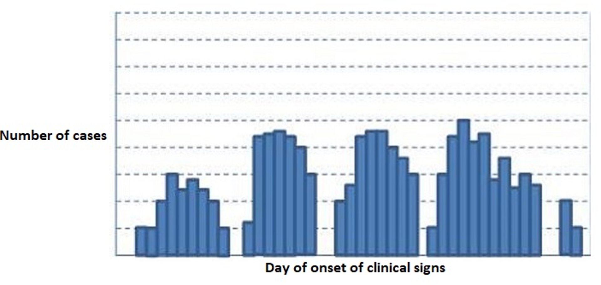
Epidemic curve for a hypothetical common source outbreak with intermittent exposure (eg, intermittent access to a play yard contaminated with roundworm and hookworm eggs). Case numbers peak at irregular times corresponding to the earlier exposures. The x-axis represents the day of onset of clinical signs and the y-axis represents the number of cases.
Courtesy of Dr. Donald L. Noah.

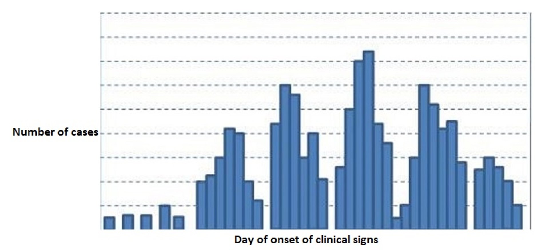
Epidemic curve for a hypothetical propagated source outbreak in which cases can directly infect other cases separate from the initial source (eg, contagious disease). In a propagated source outbreak, individual-to-individual transmission occurs, often through several cycles before declining. The x-axis represents the day of onset of clinical signs and the y-axis represents the number of cases.
Courtesy of Dr. Donald L. Noah.
Establishing a working case definition is the method by which public health officials define what individuals are included as official cases in the outbreak and illustrate the boundaries of the outbreak. An effective case definition is critical because it may be confusing, especially in the absence of definitive diagnostics, to differentiate between actual disease cases and those ill from other causes. The case definition defines a case in terms of person, place, and time. Person criteria typically include vulnerability factors such as age, sex, clinical signs, or exposure history. Place criteria usually include a geographic boundary such as a state or local area, a farm, or a particular shelter. Time parameters may be after an implicated meal (if foodborne) or other types of exposures. Case definitions are usually based on either clinical signs or diagnostic test results. The former is more subjective than the latter but can be just as effective, especially in field epidemiological conditions. As the investigation ensues and more information becomes available, it may be necessary to revise the case definition. However, this is done judiciously, because changes to the case definition result in changes to how the data are interpreted.
The epidemic curve (epi curve) is a simple plot of the number of affected animals in a population over time and is an important tool to describe the progression of an outbreak. The horizontal axis represents a time interval (usually the date when an individual developed clinical signs, also called the date of onset). The vertical axis is the number of new cases on each date. These are updated as new data come in and thus are subject to change. The epidemic curve is complex and may be limited by information deficiencies and inaccurate case definitions. Despite these potential limitations, detailed information regarding the dates and numbers of reported cases is visually useful. Moreover, in addition to the magnitude and duration of the outbreak, the shape of the curve can show useful information regarding the nature of the outbreak.
The overall shape of the epidemic curve can give clues to the type of exposure that resulted in the outbreak. Typical epidemic curves from common sources include a common specific point source in which all cases were exposed at the same time and place (eg, a foodborne illness outbreak); a common source with continuous exposure in which although the source is common, cases gradually rise before either peaking or plateauing and declining; and a common source with intermittent exposure in which the peaks occur at irregular times corresponding to the earlier exposures. In addition to outbreaks having common sources, they can have propagated sources, in which cases can directly infect other cases separate from the initial source. In a propagated source outbreak, individual-to-individual transmission occurs, often through several cycles before declining.
Another attribute of an outbreak that can be illustrated by the epidemic curve is the incubation period (the time from infection to the onset of signs [or positive test results]). In a common point source outbreak, the peak of cases occurs one incubation period after the exposure event. In a propagated source outbreak, the peaks of cases occur one incubation period apart. Based on known minimum and maximum incubation periods, the most likely period of exposure can be identified for investigators to focus on when searching for the event when the exposure occurred (eg, a new bag of feed or exposure to an infected individual).
In a propagated (or infectious) disease outbreak, the number of secondary cases that typically result from each new case is termed the effective reproduction number, symbolized as R. Assuming no other individuals are infected or immunized (naturally or through vaccination), mathematical models can estimate the expected number of cases directly generated by one case in a wholly susceptible population, termed the basic reproduction number, symbolized as R0 (often pronounced as "R naught"). By definition, therefore, R0 cannot be modified through vaccination campaigns. Note that R0 is a dimensionless number and not a rate, which would have units of time.
For More Information
Giuffrida MA. Defining the primary research question in veterinary clinical studies. J Am Vet Med Assoc. 2016;249(5):547-551.
Cernicchiaro N, Oliveira ARS, Hanthorn C. Outcomes research: origins, relevance, and potential impacts for veterinary medicine.J Am Vet Med Assoc. 2022;260(7):714-723.